Datetime inputs

Datetime inputs of the following types are supported in PyGMT:

• numpy.datetime64

• pandas.DatetimeIndex

• xarray.DataArray: datetimes included in an xarray.DataArray

• raw datetime strings in ISO 8601 format (e.g. "YYYY-MM-DD", "YYYY-MM-DDTHH", and "YYYY-MM-DDTHH:MM:SS")

• Python built-in datetime.datetime and datetime.date

We can pass datetime inputs based on one of the types listed above directly to the x and y parameters of e.g. the pygmt.Figure.plot method.

The region parameter has to include the \(x\) and \(y\) axis limits in the form [date_min, date_max, ymin, ymax]. Here date_min and date_max can be directly defined as datetime input.

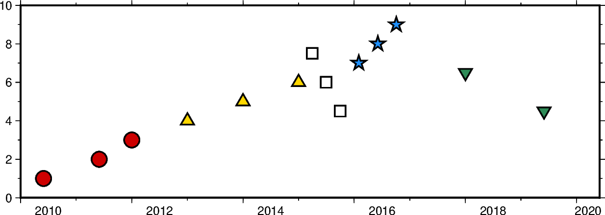
import datetime as dt

import numpy as np
import pandas as pd
import pygmt
import xarray as xr
from pygmt.params import Axis, Frame

fig = pygmt.Figure()

# create a basemap with limits of 2010-01-01 to 2020-06-01 on the x-axis and
# 0 to 10 on the y-axis
fig.basemap(
    projection="X15c/5c",
    region=[dt.date(2010, 1, 1), dt.date(2020, 6, 1), 0, 10],
    frame=Frame(axes="WSen", axis=Axis(annot=True, tick=True)),
)

# numpy.datetime64 types
x = np.array(
    ["2010-06-01", "2011-06-01T12", "2012-01-01T12:34:56"], dtype=np.datetime64
)
y = [1, 2, 3]
fig.plot(x=x, y=y, style="c0.4c", pen="1p", fill="red3")

# pandas.DatetimeIndex
x = pd.date_range("2013", periods=3, freq="YS")
y = [4, 5, 6]
fig.plot(x=x, y=y, style="t0.4c", pen="1p", fill="gold")

# xarray.DataArray
x = xr.DataArray(data=pd.date_range(start="2015-03", periods=3, freq="QS"))
y = [7.5, 6, 4.5]
fig.plot(x=x, y=y, style="s0.4c", pen="1p")

# raw datetime strings
x = ["2016-02-01", "2016-06-04T14", "2016-10-04T00:00:15"]
y = [7, 8, 9]
fig.plot(x=x, y=y, style="a0.4c", pen="1p", fill="dodgerblue")

# the Python built-in datetime and date
x = [dt.date(2018, 1, 1), dt.datetime(2019, 6, 1, 20, 5, 45)]
y = [6.5, 4.5]
fig.plot(x=x, y=y, style="i0.4c", pen="1p", fill="seagreen")

fig.show()